Letter Segmentation and OCR
Thanks to your work on homework03 and homework04, the police were
able to fully extract the text from the kidnapping letters:
"v ybirq zheqrevat ze gurvfrasyblq ng gur rfgngr gur tnf jnf gur cresrpg zheqre jrncba vz fher vyy trg njnl jvgu vg nf jryy ubcrshyyl abobql svtherf bhg gur pbzovangvba bs gur cnqybpx cynl ba ybpxre 69 ba gur frpbaq sybbe bs phfuvat bgurejvfr v nz va erny gebhoyr"
(This is not the actual text, the original cipher I chose to
encode the kidnapping letters ended up being way too hard for a seq2seq
model to break, which is great for the field of cryptography but kind of
embarrassing for AI)
Unfortunately, it appears that the text has been encoded somehow! As
you try to recover from pigtostal (swimming lost the houses for that
right?) you realize that maybe you could treat this as a machine
translation task. You could pretend the cipher is the source language
and the plaintext is the target language.
If you could figure out the cipher then you could generate a training
set of (cipher, plaintext) pairs. You could then train a seq2seq model
to translate the ciphertext into plaintext!
letter_text = "v ybirq zheqrevat ze gurvfrasyblq ng gur rfgngr gur tnf jnf gur cresrpg zheqre jrncba vz fher vyy trg njnl jvgu vg nf jryy ubcrshyyl abobql svtherf bhg gur pbzovangvba bs gur cnqybpx cynl ba ybpxre 69 ba gur frpbaq sybbe bs phfuvat bgurejvfr v nz va erny gebhoyr"
Text Similarity
Your first step is to figure out which cipher was most likely used to
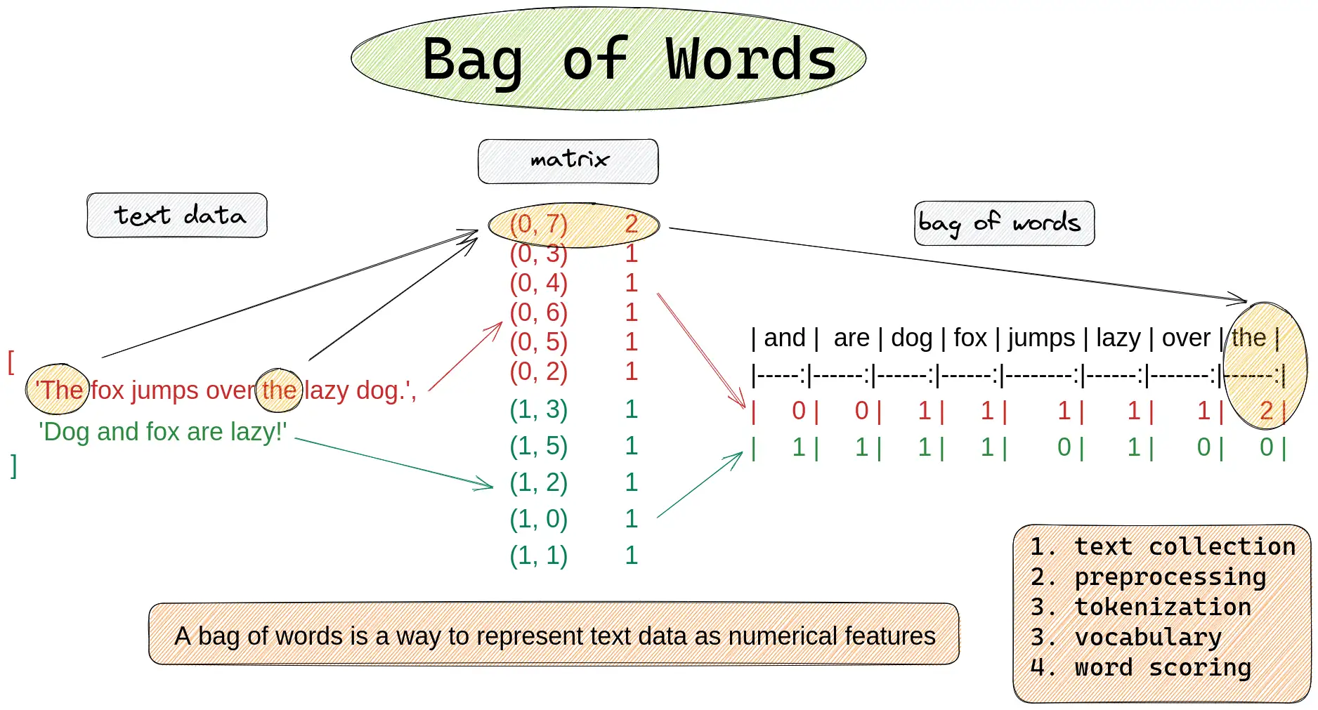
encode the kidnapping letters. To do this, you should test a Bag of
Words and a Bag of Characters similarity metric. As with most of machine
learning, we need to somehow convert our text into a vector to allow us
to compare it to other vectors. One option would be to use a pre-trained
embedding network like word2vec or GloVe (this would be like using the
output of convolutional layers as features for MNIST). However, for now
we will just use a Bag of Words and an N-Gram model instead (much
simpler).
Bag of Words

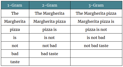
N-Grams
If you can remember all the way back to lecture07: Markov Models,
you'll remember that we've actually seen these before, in the context of
a Markov Babbler!

However for this task, I'd recommend using a character level N-Gram
model instead, as we just want to compare character frequencies, it's
tough to predict how ciphers will modify words and there's unlikely to
be any overlap between the two.
Ciphers
Your task will be to use the following ciphers to encode some basic
text, and then implement BoW and character level N-Gram similarity
functions to try and figure out which cipher was most likely used to
encode the kidnapping letters.
The ciphers to test are: Caesar, Vigenère, Substitution, Affine, and
ROT13.
import string
import math
from collections import Counter

# -------------------------------
# CIPHER IMPLEMENTATIONS
# -------------------------------

def caesar_cipher(text, shift):
    """Encode text using a Caesar cipher with the specified shift."""
    result = ""
    for char in text:
        if char.isalpha():
            base = 'A' if char.isupper() else 'a'
            result += chr((ord(char) - ord(base) + shift) % 26 + ord(base))
        else:
            result += char
    return result

def rot13(text):
    """Encode text using ROT13 (a Caesar cipher with shift 13)."""
    return caesar_cipher(text, 13)

def vigenere_cipher(text, keyword):
    """Encode text using the Vigenère cipher with a given keyword."""
    result = ""
    keyword = keyword.lower()
    keyword_length = len(keyword)
    j = 0  # index for keyword letters
    for char in text:
        if char.isalpha():
            base = 'A' if char.isupper() else 'a'
            # Determine shift amount from the keyword character
            shift = ord(keyword[j % keyword_length]) - ord('a')
            result += chr((ord(char) - ord(base) + shift) % 26 + ord(base))
            j += 1
        else:
            result += char
    return result

def substitution_cipher(text, mapping):
    """
    Encode text using a substitution cipher defined by the given mapping.
    'mapping' should be a dictionary mapping each lowercase letter to its substitute.
    """
    result = ""
    for char in text:
        if char.isalpha():
            if char.isupper():
                # Convert to lower case, substitute, then convert back to upper case
                sub = mapping.get(char.lower(), char.lower()).upper()
            else:
                sub = mapping.get(char, char)
            result += sub
        else:
            result += char
    return result

def affine_cipher(text, a, b):
    """
    Encode text using an Affine cipher with parameters a and b.
    The function assumes that a and 26 are coprime.
    """
    result = ""
    for char in text:
        if char.isalpha():
            base = 'A' if char.isupper() else 'a'
            x = ord(char) - ord(base)
            # Apply the affine transformation: E(x) = (a * x + b) mod 26
            y = (a * x + b) % 26
            result += chr(y + ord(base))
        else:
            result += char
    return result

# -------------------------------
# FEATURE COMPARISON FUNCTIONS
# -------------------------------

def one_gram_similarity(text1, text2):
    """
    Computes the cosine similarity between two texts based on character frequencies.
    Only considers alphanumeric characters after converting to lower case.
    """

    #TODO: Calculate 1-gram character frequencies and use cosine similarity between the two vectors

    return dot_product / (norm1 * norm2)

def bow_similarity(text1, text2):
    """
    Computes the cosine similarity between two texts based on word frequencies.
    Splits the text on whitespace after converting to lower case.
    """

    #TODO: Calculate bag of words and use cosine similarity between the two vectors

    return dot_product / (norm1 * norm2)
# Sample Lorem Ipsum text
text = ("Lorem ipsum dolor sit amet, consectetur adipiscing elit, sed do eiusmod tempor "
        "incididunt ut labore et dolore magna aliqua.")
print("Original text:")
print(text)

# Encode using different ciphers
caesar_encoded = caesar_cipher(text, 3)  # Caesar with shift 3
vigenere_encoded = vigenere_cipher(text, "key")  # Vigenère with keyword 'key'

# Substitution cipher: define a substitution mapping (e.g., a scrambled alphabet)
alphabet = string.ascii_lowercase
# Example mapping using a predetermined scramble. (For real use, ensure this mapping is a permutation.)
subs_alphabet = "qwertyuiopasdfghjklzxcvbnm"
mapping = {alphabet[i]: subs_alphabet[i] for i in range(26)}
substitution_encoded = substitution_cipher(text, mapping)

affine_encoded = affine_cipher(text, 5, 8)  # Affine with a=5 and b=8
rot13_encoded = rot13(text)  # ROT13

# Show the encoded texts
print("\nEncoded texts:")
print("Caesar Cipher:      ", caesar_encoded)
print("Vigenère Cipher:    ", vigenere_encoded)
print("Substitution Cipher:", substitution_encoded)
print("Affine Cipher:      ", affine_encoded)
print("ROT13:              ", rot13_encoded)

letter_string = "v ybirq zheqrevat ze gurvfrasyblq ng gur rfgngr gur tnf jnf gur cresrpg zheqre jrncba vz fher vyy trg njnl jvgu vg nf jryy ubcrshyyl abobql svtherf bhg gur pbzovangvba bs gur cnqybpx cynl ba ybpxre 69 ba gur frpbaq sybbe bs phfuvat bgurejvfr v nz va erny gebhoyr"

print('Kidnapping letter text:', letter_string)

# Save the encoded texts in a dictionary for easy iteration
encoded_versions = {
    "Caesar": caesar_encoded,
    "Vigenère": vigenere_encoded,
    "Substitution": substitution_encoded,
    "Affine": affine_encoded,
    "ROT13": rot13_encoded
}

#TODO: For each cipher, calculate the BoW and 1-gram similarity with the letter string to figure out which cipher was used

print("\nBag-of-Words (BoW) similarity with test string:")


print("\nBag-of-Characters (BoC) similarity with test string:")
Expected Output
Original text:
Lorem ipsum dolor sit amet, consectetur adipiscing elit, sed do eiusmod tempor incididunt ut labore et dolore magna aliqua.

Encoded texts:
Caesar Cipher:       Oruhp lsvxp groru vlw dphw, frqvhfwhwxu dglslvflqj holw, vhg gr hlxvprg whpsru lqflglgxqw xw oderuh hw groruh pdjqd doltxd.
Vigenère Cipher:     Vspoq gzwsw hmvsp cmr kqcd, gmxwcmxcdyp khgzmqmmlq ijsx, qoh by igewkyh roqnyv gxggnmberr ex jkfmbi cd hmvspo qyqry kpgayy.
Substitution Cipher: Sgktd ohlxd rgsgk loz qdtz, egflteztzxk qroholeofu tsoz, ltr rg toxldgr ztdhgk ofeororxfz xz sqwgkt tz rgsgkt dqufq qsojxq.
Affine Cipher:       Lapcq wfueq xalap uwz iqcz, savucszczep ixwfwuswvm clwz, ucx xa cweuqax zcqfap wvswxwxevz ez linapc cz xalapc qimvi ilwkei.
ROT13:               Yberz vcfhz qbybe fvg nzrg, pbafrpgrghe nqvcvfpvat ryvg, frq qb rvhfzbq grzcbe vapvqvqhag hg ynober rg qbyber zntan nyvdhn.
Kidnapping letter text: v ybirq zheqrevat ze gurvfrasyblq ng gur rfgngr gur tnf jnf gur cresrpg zheqre jrncba vz fher vyy trg njnl jvgu vg nf jryy ubcrshyyl abobql svtherf bhg gur pbzovangvba bs gur cnqybpx cynl ba ybpxre 69 ba gur frpbaq sybbe bs phfuvat bgurejvfr v nz va erny gebhoyr

Bag-of-Words (BoW) similarity with test string:
  Caesar      : 0.0000
  Vigenère    : 0.0000
  Substitution: 0.0000
  Affine      : 0.0000
  ROT13       : 0.0000

Bag-of-Characters (BoC) similarity with test string:
  Caesar      : 0.6023
  Vigenère    : 0.6518
  Substitution: 0.5527
  Affine      : 0.4254
  ROT13       : 0.9198
It definitely looks like the text was a ROT13 cipher! Now we could of
course just directly use the ROT13 cipher to decode the text, but
where's the fun in that? AI is the future right! You're using it to
replace your ability to do even the most basic thinking tasks so
obviously we should also use it here instead of just the closed form
solution!
What we need to do now is create a dataset of (ciphertext, plaintext)
pairs to train a seq2seq model to decode the ciphertext. Luckily, we can
use a library called NLTK to get a list of words in the English
language. We can use this list to generate a dataset of (ciphertext,
plaintext) pairs.
NLTK: Natural Language Toolkit is
one of the most popular libraries for working with text in
Python. It's a great tool to have in your toolbelt.
In the cell below lets create our dataset of (ciphertext, plaintext)
pairs, start with 100000 pairs and lets see how well the model does.
import torch
import torch.nn as nn
import torch.optim as optim
from torch.utils.data import Dataset, DataLoader
from torch.nn.utils.rnn import pad_sequence
import nltk
import codecs
import numpy as np

# ---------------------
# 1. Data Preparation
# ---------------------

# Download the NLTK 'words' corpus if needed.
nltk.download('words')
from nltk.corpus import words

# Fixed vocabulary: <PAD> token plus 26 lowercase letters.
vocab = ['<PAD>'] + ['<EOS>'] + ['<UNK>'] + ['<SOS>'] + [' '] + list("abcdefghijklmnopqrstuvwxyz")
vocab_size = len(vocab)  # should be 27
char2idx = {ch: idx for idx, ch in enumerate(vocab)}
idx2char = {idx: ch for idx, ch in enumerate(vocab)}
padding_idx = char2idx['<PAD>']

# Custom Dataset: each example is a tuple (rot13_word, original_word)
class Rot13Dataset(Dataset):
    def __init__(self, word_list, char2idx):
        self.data = []
        for word in word_list:
            # Only consider fully alphabetic words.
            if word.isalpha():
                word = word.lower()
                rot13_word = codecs.encode(word, 'rot_13')
                input_seq = torch.tensor([char2idx[c] for c in rot13_word], dtype=torch.long)
                target_seq = torch.tensor([char2idx[c] for c in word], dtype=torch.long)
                self.data.append((input_seq, target_seq))

    def __len__(self):
        return len(self.data)

    def __getitem__(self, idx):
        return self.data[idx]

# Collate function to pad sequences.
def collate_fn(batch):
    inputs, targets = zip(*batch)
    inputs_padded = pad_sequence(inputs, batch_first=True, padding_value=padding_idx)
    targets_padded = pad_sequence(targets, batch_first=True, padding_value=padding_idx)
    return inputs_padded, targets_padded

# Get words from NLTK and take a subset.
word_list = words.words()
filtered_words = [w for w in word_list if w.isalpha()]
subset_words = filtered_words[:100000]

dataset = Rot13Dataset(subset_words, char2idx)
dataloader = DataLoader(dataset, batch_size=64, shuffle=True, collate_fn=collate_fn)
print(f"Total training samples: {len(dataset)}")
Numpy RNN Model
Given this dataset, we now need a seq2seq model to decode the
ciphertext. We'll start with a simple RNN model that you'll need to
implement in numpy

Remember that unlike a FFN, data in an RNN loops around over the
sequence of inputs, to allow us to build up a hidden state (context in
my words) that can be used to generate the next output. There's a really
good cheatsheet
from Stanford about RNNs that I'd recommend.
class Tanh:
    def __init__(self):
       # TODO: Implement Tanh activation function
       pass

    def forward(self, x):
        # TODO: Implement forward pass for Tanh activation function
        pass

    def backward(self, x):
        # TODO: Implement backward pass for Tanh activation function
        pass

    def update(self, lr):
        # TODO: Implement update function for Tanh activation function
        pass

# ---------------------
# Fully Connected (Linear) Layer (for final projection)
# ---------------------
class LinearLayer:
    def __init__(self, input_dim, output_dim):
        # TODO: Implement initialization for LinearLayer
        pass

    def forward(self, X):
        # TODO: Implement forward pass for LinearLayer
        pass

    def backward(self, dA):
        # TODO: Implement backward pass for LinearLayer
        pass

    def update(self, lr):
        # TODO: Implement update function for LinearLayer
        pass

class LinearContextLayer:
    def __init__(self, input_dim, hidden_size):
        # TODO: Implement initialization for LinearContextLayer
        pass

    def forward(self, X):
        # TODO: Implement forward pass for LinearContextLayer
        pass

    def backward(self, d_outputs):
        # TODO: Implement backward pass for LinearContextLayer
        pass

    def update(self, lr):
        # TODO: Implement update function for LinearContextLayer
        pass

# ---------------------
# Embedding Layer
# ---------------------
class EmbeddingLayer:
    def __init__(self, vocab_size, embed_size):
        self.W = np.random.randn(vocab_size, embed_size) * 0.01

    def forward(self, x):
        return self.W[x]

# ---------------------
# Complete Numpy RNN Model
# ---------------------
class NumpyClassRNN:
    def __init__(self, vocab_size, embed_size, hidden_size, padding_idx=0):
        self.vocab_size = vocab_size
        self.embed_size = embed_size
        self.hidden_size = hidden_size
        self.padding_idx = padding_idx

        # Layers:
        self.embedding = EmbeddingLayer(vocab_size, embed_size)

        # For the recurrent context layer, the input dimension is the embed_size.
        self.context = LinearContextLayer(embed_size, hidden_size)

        # Final fully connected layer: project hidden state to vocabulary logits.
        self.linear = LinearLayer(hidden_size, vocab_size)

        # Keep model layers in a list for easy backward and update passes.
        self.model = [self.context, self.linear]

    def forward(self, x):
        """
        Args:
          x: (batch_size, seq_len) with integer token indices.
        Returns:
          logits: (batch_size, seq_len, vocab_size)
          outputs: (batch_size, seq_len, hidden_size) final hidden states over time.
        """

        # TODO: Implement forward pass for NumpyClassRNN

        return self.logits, self.outputs

    def backward(self, d_logits, learning_rate=0.001):
       # TODO: Implement backward pass for NumpyClassRNN
       pass

# ---------------------
# Loss Function (Cross-Entropy) and Gradient
# ---------------------
def cross_entropy_loss_and_grad(logits, targets, padding_idx):
    """
    Computes cross-entropy loss and its gradient.

    Args:
      logits: (batch_size, seq_len, vocab_size)
      targets: (batch_size, seq_len) integer indices.
      padding_idx: token index for padding to be ignored.

    Returns:
      loss: scalar loss averaged over the batch.
      d_logits: gradient of loss with respect to logits.
    """

    # TODO: Implement cross-entropy loss and gradient

    return loss, d_logits

# ---------------------
# 4. Training Loop (NumPy version)
# ---------------------

# Instantiate our NumPy-based RNN.
model = NumpyClassRNN(vocab_size=vocab_size, embed_size=32, hidden_size=64, padding_idx=padding_idx)

num_epochs = 100
learning_rate = 0.001

# TODO: Implement training loop
for epoch in range(num_epochs):
   pass
My training output
Training time: 5m 21.2s
Epoch 1/100 - Loss: 28.0207
Epoch 26/100 - Loss: 16.5287
Epoch 51/100 - Loss: 6.4490
Epoch 76/100 - Loss: 3.0717
This is extremely approximate output of what you should expect.
Cracking the kidnapping
letter cipher
Now that we have our trained RNN, we can use the kidnapping
ciphertext as our input and see if we can decode it!
# ---------------------
# 5. Testing / Prediction Function
# ---------------------

def predict(model, input_str, char2idx, idx2char):
    # TODO: Implement prediction function for each word  in the input string
    pass

    return predicted_str

kidnapping_letter = "v ybirq zheqrevat ze gurvfrasyblq ng gur rfgngr gur tnf jnf gur cresrpg zheqre jrncba vz fher vyy trg njnl jvgu vg nf jryy ubcrshyyl abobql svtherf bhg gur pbzovangvba bs gur cnqybpx nopqr ba ybpxre ba gur frpbaq sybbe bs svgm bgurejvfr v nz va erny gebhoyr"

predicted_original = predict(model, kidnapping_letter, char2idx, idx2char)
print(f"Input (ROT13): {kidnapping_letter}")
print(f"Predicted original: {predicted_original}")
I'm not going to show you the expected out of the kidnapping letter
as that'd spoil some of the surprise but absolutely do NOT expect to get
perfectly clean english out of this, I could make out most of the words
but it's pretty garbled and unfortunately because it's not perfect we
can't quite get the correct padlock combination from it. However,
chatGPT is of course the greatest thing since sliced bread, so maybe if
we use a transformer model it will do better! It's what's already doing
this homework for you, surely it can also crack the kidnapping letter
cipher!
Now that we have a working RNN model, let's try training a
Transformer model to see if it can do any better. For the transformer
we'll just be using the pytorch implementation of one. We'll need to set
up our dataset a little differently, but that's been done for you. My
model trained for about an 60 minutes with approximately 270,000 pairs
and I still couldn't get a perfect translation. Don't feel like you have
to let yours train for that long, feel free to use a smaller dataset,
but you will get significantly worse results.
import torch
import torch.nn as nn
import torch.optim as optim
from torch.utils.data import Dataset, DataLoader
from torch.nn.utils.rnn import pad_sequence
import nltk
import codecs

# ---------------------
# 1. Data Preparation
# ---------------------

# Download the NLTK 'words' corpus if needed.
nltk.download('words')
from nltk.corpus import words

# Fixed vocabulary: <PAD>, <EOS>, <UNK>, <SOS>, space, and 26 lowercase letters.
vocab = ['<PAD>', '<EOS>', '<UNK>', '<SOS>', ' '] + list("abcdefghijklmnopqrstuvwxyz")
vocab_size = len(vocab)  # should be 31 (if 4 specials + space + 26 letters)
char2idx = {ch: idx for idx, ch in enumerate(vocab)}
idx2char = {idx: ch for idx, ch in enumerate(vocab)}
padding_idx = char2idx['<PAD>']

# Custom Dataset: each example is a tuple (rot13_word, original_word)
class Rot13Dataset(Dataset):
    def __init__(self, word_list, char2idx):
        self.data = []
        for word in word_list:
            # Only consider fully alphabetic words.
            if word.isalpha():
                word = word.lower()
                rot13_word = codecs.encode(word, 'rot_13')
                # Create input sequence from the ROT13 word.
                input_seq = torch.tensor(
                    [char2idx.get(c, char2idx['<UNK>']) for c in rot13_word],
                    dtype=torch.long
                )
                # Create target sequence from the original word.
                target_seq = torch.tensor(
                    [char2idx.get(c, char2idx['<UNK>']) for c in word],
                    dtype=torch.long
                )
                self.data.append((input_seq, target_seq))

    def __len__(self):
        return len(self.data)

    def __getitem__(self, idx):
        input_seq, target_seq = self.data[idx]
        # Prepare decoder input by prepending <SOS>
        tgt_input = torch.cat([torch.tensor([char2idx['<SOS>']], dtype=torch.long), target_seq])
        # Prepare decoder output by appending <EOS>
        tgt_output = torch.cat([target_seq, torch.tensor([char2idx['<EOS>']], dtype=torch.long)])
        return input_seq, tgt_input, tgt_output

# Collate function to pad sequences.
def collate_fn(batch):
    # Each sample now is a triple: (input_seq, tgt_input, tgt_output)
    inputs, tgt_inputs, tgt_outputs = zip(*batch)
    inputs_padded = pad_sequence(inputs, batch_first=True, padding_value=padding_idx)
    tgt_inputs_padded = pad_sequence(tgt_inputs, batch_first=True, padding_value=padding_idx)
    tgt_outputs_padded = pad_sequence(tgt_outputs, batch_first=True, padding_value=padding_idx)
    return inputs_padded, tgt_inputs_padded, tgt_outputs_padded

# Get words from NLTK and take a subset.
word_list = words.words()
filtered_words = [w for w in word_list if w.isalpha()]
subset_words = filtered_words[:1000]

dataset = Rot13Dataset(subset_words, char2idx)
dataloader = DataLoader(dataset, batch_size=64, shuffle=True, collate_fn=collate_fn)
print(f"Total training samples: {len(dataset)}")
import math
import torch
import torch.nn as nn
import torch.optim as optim

class PositionalEncoding(nn.Module):
    def __init__(self, d_model, max_len):
         super(PositionalEncoding, self).__init__()
         pe = torch.zeros(max_len, d_model)
         position = torch.arange(0, max_len, dtype=torch.float).unsqueeze(1)
         div_term = torch.exp(torch.arange(0, d_model, 2).float() * (-math.log(10000.0) / d_model))
         pe[:, 0::2] = torch.sin(position * div_term)
         pe[:, 1::2] = torch.cos(position * div_term)
         pe = pe.unsqueeze(0)  # shape (1, max_len, d_model)
         self.register_buffer('pe', pe)

    def forward(self, x):
         # x has shape (batch, seq_len, d_model)
         # Ensure that the positional encodings cover the maximum possible length
         x = x + self.pe[:, :x.size(1)]
         return x

# -----------------------------
# 4. Build the Transformer Model
# -----------------------------
class Rot13Transformer(nn.Module):
    def __init__(self, vocab_size, d_model, nhead, num_encoder_layers,
                 num_decoder_layers, dim_feedforward, dropout, max_len):
         super(Rot13Transformer, self).__init__()

        # TODO: Implement initialization for Rot13Transformer

    def forward(self, src, tgt, src_mask=None, tgt_mask=None,
                src_key_padding_mask=None, tgt_key_padding_mask=None):

         #TODO: Implement forward pass for Rot13Transformer
            #TODO: Embed and scale the source tokens
            #TODO: Embed and scale the target tokens
            #TODO: Note: Transformer expects input shape (seq_len, batch, d_model) so we transpose
            #TODO: Transpose back and pass through final linear layer to obtain vocabulary logits

         return output

# Helper function to create a subsequent mask for the decoder (to prevent access to future tokens)
def generate_square_subsequent_mask(sz):
    mask = torch.triu(torch.ones(sz, sz) == 1).transpose(0, 1)
    mask = mask.float().masked_fill(mask == 0, float('-inf')).masked_fill(mask == 1, float(0.0))
    return mask
dataset = Rot13Dataset(subset_words, char2idx)
dataloader = DataLoader(dataset, batch_size=64, shuffle=True, collate_fn=collate_fn)

device = torch.device("cuda" if torch.cuda.is_available() else "cpu")
max_len = 100

# Initialize the transformer model with hyperparameters
model = Rot13Transformer(
    vocab_size=vocab_size,
    d_model=128,
    nhead=4,
    num_encoder_layers=2,
    num_decoder_layers=2,
    dim_feedforward=256,
    dropout=0.1,
    max_len=max_len
)
model = model.to(device)

optimizer = optim.Adam(model.parameters(), lr=0.001)
criterion = nn.CrossEntropyLoss(ignore_index=padding_idx)

model.train()
for epoch in range(num_epochs):
    #TODO: Implement training loop
    pass
My training output
Training time: 63m 1.3s
Epoch 1, Loss: 0.5194
Epoch 2, Loss: 0.0822
Epoch 3, Loss: 0.0467
Epoch 4, Loss: 0.0357
Epoch 5, Loss: 0.0279
Epoch 6, Loss: 0.0236
Epoch 7, Loss: 0.0197
Epoch 8, Loss: 0.0181
Epoch 9, Loss: 0.0161
Epoch 10, Loss: 0.0150
Epoch 11, Loss: 0.0136
Epoch 12, Loss: 0.0126
Epoch 13, Loss: 0.0115
Epoch 14, Loss: 0.0105
Epoch 15, Loss: 0.0105
Epoch 16, Loss: 0.0099
Epoch 17, Loss: 0.0092
Epoch 18, Loss: 0.0083
Epoch 19, Loss: 0.0088
Epoch 20, Loss: 0.0078
Epoch 21, Loss: 0.0070
Epoch 22, Loss: 0.0070
Epoch 23, Loss: 0.0068
Epoch 24, Loss: 0.0066
Epoch 25, Loss: 0.0065
def translate_word_by_word(model, text, char2idx, idx2char, max_len):
    model.eval()
    # Split the input text into words using whitespace
    words = text.split()
    translated_words = []

    for word in words:
        pass
        #TODO: Preprocess each word: lowercase and convert each character to its index,
        #TODO: mapping any unknown char to <UNK> (if available)
        #TODO: Pad or truncate to max_len

        #TODO: Decoder starts with the <SOS> token

        #TODO: Autoregressive decoding loop: generate one token at a time for this word

        #TODO: Convert predicted indices into characters and filter out special tokens

    #TODO: Join the translated words into a complete sentence
    return None

kidnapping_letter = "v ybirq zheqrevat ze gurvfrasyblq ng gur rfgngr gur tnf jnf gur cresrpg zheqre jrncba vz fher vyy trg njnl jvgu vg nf jryy ubcrshyyl abobql svtherf bhg gur pbzovangvba bs gur cnqybpx cynl ba ybpxre 69 ba gur frpbaq sybbe bs phfuvat bgurejvfr v nz va erny gebhoyr"

translated = translate_word_by_word(model, kidnapping_letter, char2idx, idx2char, max_len)
print("ROT13 Input:", kidnapping_letter)
print("Translated (English):", translated)
Expected Output
I trained the model for about an hour with 270,000 pairs and still
was unable to get a perfect translation. There are tricks you can play
with the model at inference time to do it, but I don't expect you to do
that.
AI Falling Short
DAMN! After all of this, AI still can't crack the kidnapping letter
cipher! Defeated by a simple rot13 cipher, the dumbest of all ciphers!
Accepting defeat, you still need to solve the murder! Unfortunately, all
we have to do is run the ciphertext back through the rot13 function to
get the original message!
rot13_text = rot13("v ybirq zheqrevat ze gurvfrasyblq ng gur rfgngr gur tnf jnf gur cresrpg zheqre jrncba vz fher vyy trg njnl jvgu vg nf jryy ubcrshyyl abobql svtherf bhg gur pbzovangvba bs gur cnqybpx cynl ba ybpxre 69 ba gur frpbaq sybbe bs phfuvat bgurejvfr v nz va erny gebhoyr")

print("ROT13 Output:", rot13_text)
Maybe sometimes we just shouldn't use AI to solve problems. Something
to think about.
Final Task
Now that you have the code for the locker, hopefully you have enough
to put this villain behind bars! Head over to the locker and open it,
take a picture of the evidence and yourselves and submit it along with
your code, the TAs will handle the police report! Remember, this is an
active investigation and tampering with the evidence will result in a
felony charge!


