Now that you have the segmented letters from the previous task, we need a way to actually convert the letters to text! You can't be bothered to just transcribe the images yourself, but you remember your professor droning on about something called MNIST and you think that these letters might be kind of similar to handwritten digits.
Unfortunately, because your professor hates you, he's making you write a FFN using only numpy for the first part of this assignment. Use the dataset available from the following link for training, testing, and validation on this assignment. Alphabet Cuttings Dataset
The code immediately below is for loading and formatting the dataset. You don't have to do anything here yourself.
import cv2
import numpy as np
import matplotlib.pyplot as plt
from PIL import Image
def detect_rgb_contours(input_path, display=False):
"""
Detect contours in the RGB channels of a PNG image and draw all contours in hierarchy.
Args:
input_path (str): Path to the input PNG image
line_thickness (int): Thickness of contour lines in pixels
"""
# Read the image with alpha channel
= cv2.imread(input_path, cv2.IMREAD_UNCHANGED)
img
# Extract the RGB channels
= img[:, :, :3]
rgb_img
# Convert to grayscale for contour detection
= cv2.cvtColor(rgb_img, cv2.COLOR_BGR2GRAY)
gray if display:
display(Image.fromarray(gray))
# Setting parameter values
= 50 # Lower Threshold
t_lower = 150 # Upper threshold
t_upper
# Applying the Canny Edge filter
= cv2.Canny(gray, t_lower, t_upper)
edge # Close the edges to form complete contours
if display:
display(Image.fromarray(edge))
# Find contours recursively
= cv2.findContours(edge, cv2.RETR_TREE, cv2.CHAIN_APPROX_SIMPLE)
contours, hierarchy
# Create a separate image for each contour with different colors
= np.zeros((rgb_img.shape[0], rgb_img.shape[1]), dtype=np.uint8)
mnist_img if display:
print(mnist_img.shape)
print(len(hierarchy))
print(hierarchy)
# Generate a different color for each contour based on index
for i, contour in enumerate(contours):
if i == 1:
-1, 0, thickness=cv2.FILLED)
cv2.drawContours(mnist_img, [contour], elif i % 2 == 1:
-1, 255, thickness=cv2.FILLED)
cv2.drawContours(mnist_img, [contour],
= cv2.resize(mnist_img, (28, 28))
mnist_img # Display the result with multiple contours
if display:
=(10, 10))
plt.figure(figsize='gray')
plt.imshow(mnist_img, cmap'off')
plt.axis(f"All {len(contours)} contours with unique colors")
plt.title(
plt.show()
return mnist_img
import numpy as np
from PIL import Image
import os
from collections import defaultdict
import random
from sklearn.preprocessing import LabelEncoder
from typing import Dict, Tuple
from IPython.display import display
def load_letter_dataset(data_dir: str, train_size: int = 7, test_size: int = 2, holdout_size: int = 1) -> Dict:
"""
Load and split letter dataset into train, test, and holdout sets.
"""
# Verify split sizes
assert train_size + test_size + holdout_size == 10, "Split sizes must sum to 10"
# Dictionary to store all instances of each letter
= defaultdict(list)
letter_instances
# Collect all image paths
for filename in os.listdir(data_dir):
if filename.endswith('.png') and not filename[0].isdigit():
= filename[0] # First character is the letter
letter = os.path.join(data_dir, filename)
instance_path
letter_instances[letter].append(instance_path)
= {'images': [], 'labels': []}
train_data = {'images': [], 'labels': []}
test_data = {'images': [], 'labels': []}
holdout_data
# Process each letter
for letter, instances in letter_instances.items():
# Randomly shuffle the instances
random.shuffle(instances)
# Split into train/test/holdout
= instances[:train_size]
train_paths = instances[train_size:train_size + test_size]
test_paths = instances[train_size + test_size:]
holdout_paths
# Load images and add to respective sets
for path in train_paths:
= detect_rgb_contours(path)
img 'images'].append(img)
train_data['labels'].append(letter)
train_data[
for path in test_paths:
= detect_rgb_contours(path)
img 'images'].append(img)
test_data['labels'].append(letter)
test_data[
for path in holdout_paths:
= detect_rgb_contours(path)
img 'images'].append(img)
holdout_data['labels'].append(letter)
holdout_data[
print(train_data['labels'][0], train_data['images'][0].shape)
=(10, 10))
plt.figure(figsize'images'][0], cmap='gray')
plt.imshow(train_data['off')
plt.axis(
plt.show()
# Convert to numpy arrays
for dataset in [train_data, test_data, holdout_data]:
'images'] = np.array(dataset['images'])
dataset['labels'] = np.array(dataset['labels'])
dataset[
return {
'train': train_data,
'test': test_data,
'holdout': holdout_data
}
def prepare_data(data_dict: Dict) -> Tuple[np.ndarray, np.ndarray, np.ndarray, np.ndarray]:
"""
Prepare data for FFN training:
- Preprocess all images
- Convert labels to numerical format
- Split into features (X) and labels (y)
"""
# Process training data
= np.array([img.reshape(-1) / 255 for img in data_dict['train']['images']])
X_train = np.array([img.reshape(-1) / 255 for img in data_dict['test']['images']])
X_test
# Convert labels to numerical format
= LabelEncoder()
label_encoder = label_encoder.fit_transform(data_dict['train']['labels'])
y_train = label_encoder.transform(data_dict['test']['labels'])
y_test
# Save label encoder mapping for reference
= dict(zip(label_encoder.classes_, label_encoder.transform(label_encoder.classes_)))
label_mapping print("Label mapping:", label_mapping)
return X_train, X_test, y_train, y_test
Neural Network from Scratch
Your task is to implement a simple neural network from scratch in numpy to classify the letters in the dataset following the architecture shown below.
In order to actually implement a training regime for our network, we'll need to specify a loss function that we can use to measure how well our network is doing. We'll use the cross entropy loss function as we're attempting a multiclass classification task.
Training our network will consist of two steps primarily, forward propagation and back propagation.
Forward propagation is the process of taking our input data, and passing it through the network to get a prediction.
Back propagation is the process of taking the derivative of the loss function with respect to the weights and biases, and using gradient descent to update the weights and biases.
In this gif we can see a brief outline of the forward and backward propagation steps.
Broadly speaking, forward is what gives us our prediction, and backward is what gives us the gradient of the loss function with respect to the weights and biases, and is how we update the weights to get closer to the right answer (done by minimizing the loss function).
We'll also need to implement a couple activation functions and their derivatives.
We're going to be using the ReLU activation function for our hidden layers, and a softmax function for our output layer. The softmax will allow us to map our output to a probability between 0 and 1 and from there to a class based on an argmax operation.
Here we can see both activation functions and their derivatives.
The part that most people find tricky about this is the backpropagation step.
As we've seen in class for "single layer" examples, to optimize the weights of a model using gradient descent, we can rewrite the loss function in terms of the weights and then take partial derivatives with respect to each weight.
Will multilayer networks, how do we take the derivative of the loss function with respect to the weights, if the weights in the previous layer are reliant on the weights in the layer before them?
Backpropagation is the solution to this and revolves around using the chain rule to take essentially a series of partial derivatives backwards through the network to get the gradient of the loss function with respect to the weights at each layer. We can then redistribute these gradients to update the weights of the network.
BETTER TEACHING
To be honest, your best bet is to watch the youtube videos by 3Blue1Brown. He's an incredible teacher and will do a better job than I can, along with better visualizations.
This is an introduction to neural networks using the MNIST dataset!
Then we have a great video on gradient descent.
Finally I'd recommend at least his first video on backpropagation, though you should probably watch the second too.
import numpy as np
class NumpyNeuralNetwork:
# Here we define the number and types of layers in our network
# we also include their activation functions
# TODO: You'll almost certainly need to add some more layers to get to 70% accuracy
= [
NN_ARCHITECTURE "input_dim": 784, "output_dim": 37, "activation": "relu"},
{"input_dim": 37, "output_dim": 26, "activation": "softmax"},
{
]
# Our init function just initializes the weights and biases for each layer
def __init__(self, seed = 42):
# random seed initiation
np.random.seed(seed)
# parameters storage initiation
self.params_values = {}
# iteration over network layers
for idx, layer in enumerate(self.NN_ARCHITECTURE):
# we number network layers from 1
= idx + 1
layer_idx
# extracting the number of units in layers
= layer["input_dim"]
layer_input_size = layer["output_dim"]
layer_output_size
# initiating the values of the W matrix
# and vector b for subsequent layers
self.params_values['W' + str(layer_idx)] = np.random.randn(
* 0.1
layer_output_size, layer_input_size) self.params_values['b' + str(layer_idx)] = np.random.randn(
1) * 0.1
layer_output_size,
def get_params_values(self):
return self.params_values
# TODO: Write the relu function
def relu(self, Z):
"""
Applies the ReLU (Rectified Linear Unit) activation function.
Inputs:
- Z: NumPy array of pre-activation values from a layer
Returns:
- A: NumPy array with ReLU outputs
Concept Check: Why is Z in a perceptron a number but Z in a neural network is a matrix of numbers?
Concept Check: What are the dimensions of the Z vector? Don't answer with a specific number but a generalizable statement
"""
return None
# TODO: Write the relu_backward function
def relu_backward(self, dA, Z):
"""
Perform the backward pass for the ReLU activation function.
Inputs:
- dA: Gradient of the loss with respect to the activation output (A) from the current layer
- Z: The input to the activation function of currently layer
Returns:
- dZ: Gradient of the loss with respect to the input (Z) of the current layers ReLU activation function
Concept Check: What is the purpose of setting the gradient dZ to 0 for elements where Z≤0 in the ReLU backward function?
Concept Check: What is the calculated dZ (the returned matrix) of this function used for?
"""
return None
# TODO: Write the softmax function
def softmax(self, Z):
"""
Computes the softmax activation function for the given input Z.
Inputs:
- Z : Input matrix to the softmax function
Returns:
- A probability distribution representing the likelihood of each class
Concept Check: What does the softmax function do and where is it normally used in a neural network?
"""
return None
# TODO: Write the softmax_backward function
def softmax_backward(self, dA, Z):
"""
Computes the gradient of the loss with respect to Z for a softmax activation function.
Inputs:
- dA: Gradient of the loss with respect to the output of the softmax layer
- Z: Input to the softmax function before activation
Returns:
- Gradient of the loss with respect to Z
"""
# Hint: for cross entropy loss function, softmax_backwards becames very simple (1 line)
return None
# TODO: Finish the single_layer_forward_propagation function
def single_layer_forward_propagation(self, A_prev, W_curr, b_curr, activation="relu"):
"""
Performs forward propagation for a single layer.
Parameters:
- A_prev: Activation from the previous layer
- W_curr: Weights for the current layer
- b_curr: Biases for the current layer
- activation: Activation function to apply
Returns:
- A: Activation output of the current layer
- Z_curr: linear transformation result before activation
Concept Check: Why do we return both A and Z_curr?
"""
# TODO: calculation of the input value for the activation function
# hint: this looks super similar to the perceptron equation!
= None
Z_curr
# selection of activation function
if activation == "relu":
= self.relu
activation_func elif activation == "sigmoid":
= self.sigmoid
activation_func else:
raise Exception('Non-supported activation function')
# TODO: return of calculated activation A and the intermediate Z matrix
return None
# TODO: Finish the full_forward_propagation function
def full_forward_propagation(self, X):
"""
Performs forward propagation through the entire neural network.
Inputs:
- X : input data
Returns:
- A_curr : final activation output of the network
- memory : dictionary storing intermediate A and Z values for backpropagation
"""
# creating a temporary memory to store the information needed for a backward step
= {}
memory # X vector is the activation for layer 0
= X
A_curr
# iteration over network layers
for idx, layer in enumerate(self.NN_ARCHITECTURE):
# we number network layers from 1
= idx + 1
layer_idx # transfer the activation from the previous iteration
= A_curr
A_prev
# TODO: extraction of the activation function for the current layer
= None
activ_function_curr # TODO: extraction of W for the current layer
= None
W_curr # TODO: extraction of b for the current layer
= None
b_curr # TODO: calculation of activation for the current layer
= None
A_curr, Z_curr
# saving calculated values in the memory
"A" + str(idx)] = A_prev
memory["Z" + str(layer_idx)] = Z_curr
memory[
# return of prediction vector and a dictionary containing intermediate values
return A_curr, memory
def get_cost_value(self, Y_hat, Y):
"""
Computes the cost of the neural network's predictions
Inputs:
- Y_hat: The predicted probabilities
- Y: ground truth labels
Output:
- The computed loss
Concept Check: What are the dimensions of Y_hat and Y?
"""
# number of examples
= Y_hat.shape[1]
m
# calculation of the cost according to the formula
= -1 / m * (np.dot(Y, np.log(Y_hat).T) + np.dot(1 - Y, np.log(1 - Y_hat).T))
cost return np.squeeze(cost)
# TODO: Write the convert_prob_into_class function
def convert_prob_into_class(self, probs):
"""
Converts probability values from the softmax function into discrete class predictions
Inputs:
- probs : 2D array where each col represents the predicted probability distribution
over classes for a given example
Output:
- probs_ : 1D array where each value represents the predicted class for each example
"""
= np.copy(probs)
probs_ pass
return probs_.flatten()
def get_accuracy_value(self, Y_hat, Y):
"""
Computes the accuracy of the model's predictions by comparing them with the true labels
Inputs:
- Y_hat:
- Y:
Output:
- The accuracy of the model’s predictions, which is the fraction of correctly predicted labels
"""
= self.convert_prob_into_class(Y_hat)
Y_hat_ return (Y_hat_ == Y).all(axis=0).mean()
# TODO: Write the single_layer_backward_propagation function
def single_layer_backward_propagation(self, dA_curr, W_curr, b_curr, Z_curr, A_prev, activation="relu"):
"""
Performs backward propagation for a single layer to calculate the gradients of the cost function
with respect to the weights, biases, and activations
Inputs:
- dA_curr: The gradient of the loss with respect to the activation output (A) from the current layer
- W_curr : The weights for the current layer
- b_curr : The biases for the current layer
- Z_curr : The linear transformation result (Z) before activation for the current layer
- A_prev : The activation from the previous layer
- activation : The activation function used in the current layer ("relu" or "sigmoid")
Output:
- dA_prev : The gradient of the loss with respect to the activation of the previous layer (used for backpropagation)
- dW_curr : The gradient of the cost function with respect to the weights (used for weight updates)
- db_curr : The gradient of the cost function with respect to the biases (used for bias updates)
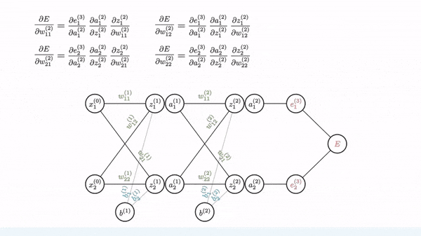
Concept Check: What is the significance of calculating dW_curr in backpropagation?
Concept Check: After calculating the gradients for weights (dW_curr) and biases (db_curr), what is the purpose
of the calculation dA_prev used for in backpropagation?
"""
# number of examples
= A_prev.shape[1]
m
# selection of activation function
if activation == "relu":
= self.relu_backward
backward_activation_func elif activation == "sigmoid":
= self.sigmoid_backward
backward_activation_func else:
raise Exception('Non-supported activation function')
# TODO: calculation of the activation function derivative
= None
dZ_curr # TODO: derivative of the matrix W
= None
dW_curr # TODO: derivative of the vector b
= None
db_curr # TODO: derivative of the matrix A_prev
= None
dA_prev
return dA_prev, dW_curr, db_curr
# TODO: Finish the full_backward_propagation function
def full_backward_propagation(self, Y_hat, Y, memory):
"""
Performs the backward propagation through the entire neural network.
Inputs:
- Y_hat: the predicted values (activations)
- Y: ground truth labels (one-hot encoded)
- memory: dictionary containing the activations and pre-activations (Z values)
for each layer during the forward pass.
Outputs:
- grads_values: dictionary containing the gradients of the cost function
with respect to the weights, biases, and activations for each layer.
Concept Check: Why store the calculated gradients in a dictionary? How will they be used?
"""
= {}
grads_values
# number of examples
= Y.shape[1]
m # a hack ensuring the same shape of the prediction vector and labels vector
= Y.reshape(Y_hat.shape)
Y
# TODO: initiation of gradient descent algorithm
# hint: The initial gradient of the loss with respect to the activation can be set up using only the the predicted labels, true lables, and one mathmatical operator
= None
dA_prev
# iteration over network layers
for layer_idx_prev, layer in reversed(list(enumerate(self.NN_ARCHITECTURE))):
# we number network layers from 1
= layer_idx_prev + 1
layer_idx_curr
# extraction of the activation function for the current layer
= layer["activation"]
activ_function_curr
= dA_prev
dA_curr
# We get the activation from the previous layer and the Z matrix from the current layer
= memory["A" + str(layer_idx_prev)]
A_prev = memory["Z" + str(layer_idx_curr)]
Z_curr
# We get the weights and biases for the current layer
= self.params_values["W" + str(layer_idx_curr)]
W_curr = self.params_values["b" + str(layer_idx_curr)]
b_curr
# TODO: calculate the gradients of the cost function with respect to the weights and biases
= None
dA_prev, dW_curr, db_curr
# We save the gradients of the cost function with respect to the weights and biases
"dW" + str(layer_idx_curr)] = dW_curr
grads_values["db" + str(layer_idx_curr)] = db_curr
grads_values[
return grads_values
def update(self, grads_values):
"""
Updates the weights and biases of the neural network during gradient descent.
Inputs:
- grads_values: dictionary containing the previously calculated gradients
Outputs:
- params_values: dictionary containing the updated values of the weights and biases
"""
# iteration over network layers
for layer_idx, layer in enumerate(self.NN_ARCHITECTURE, 1):
self.params_values["W" + str(layer_idx)] -= self.learning_rate * grads_values["dW" + str(layer_idx)]
self.params_values["b" + str(layer_idx)] -= self.learning_rate * grads_values["db" + str(layer_idx)]
return self.params_values
# TODO: Finish the train function
def train(self, X, Y, epochs=100, learning_rate=0.01, batch_size=8, verbose=False):
"""
Train the neural network using mini-batch gradient descent
Inputs:
- X: Input data (features), shape (n_features, n_examples)
- Y: True labels, shape (n_classes, n_examples)
- epochs: Number of training iterations
- learning_rate: Learning rate for gradient descent
- batch_size: Size of each mini-batch
- verbose: If True, prints cost and accuracy at intervals
Outputs:
- Dictionary containing cost and accuracy history over epochs
"""
# initiation of lists storing the history of metrics calculated during the learning process
= []
cost_history = []
accuracy_history = X.shape[1]
m
# TODO: implement mini-batch training
for i in range(epochs):
# Mini-batch processing
= np.random.permutation(m)
permutation = X[:, permutation]
X_shuffled = Y[:, permutation]
Y_shuffled
for j in range(0, m, batch_size):
#TODO: Forward propagation
pass
#TODO: Backward propagation
pass
#TODO: Update parameters
self.update(grads, learning_rate)
# TODO: Calculate metrics for the whole epoch (cost and accuracy)
# Append metrics to storage
cost_history.append(cost)
accuracy_history.append(accuracy)
if verbose and i % 500 == 0:
print(f"Epoch {i+1}/{epochs}")
print(f"Cost: {cost:.5f}")
print(f"Accuracy: {accuracy:.5f}")
print("-" * 30)
return {'cost_history': cost_history, 'accuracy_history': accuracy_history}
# Comment to prevent docstrings from being printed
The cell below will allow you to evaluate the performance of your FFN on the holdout set.
import numpy as np
def evaluate_on_holdout(data_dict, model):
"""
Evaluate the trained model on the holdout set
Args:
data_dict: Dictionary containing the dataset splits
model: Trained NumpyNeuralNetwork model
Returns:
float: Accuracy on holdout set
np.ndarray: Confusion matrix
"""
# Preprocess holdout data
= np.array([img.reshape(-1) / 255 for img in data_dict['holdout']['images']])
X_holdout
# Get labels and convert to numerical format using the same encoder
= LabelEncoder()
label_encoder 'train']['labels']) # Fit on training data to maintain same mapping
label_encoder.fit(data_dict[= label_encoder.transform(data_dict['holdout']['labels'])
y_holdout
# Convert to format needed by model
= X_holdout.T
X_holdout = np.eye(26)[y_holdout].T
y_holdout_onehot
# Get predictions
= model.full_forward_propagation(X_holdout)
y_pred, _ = model.get_accuracy_value(y_pred, y_holdout_onehot)
accuracy
# Get predicted classes
= np.argmax(y_pred, axis=0)
predicted_classes
# Create confusion matrix
from sklearn.metrics import confusion_matrix
= confusion_matrix(y_holdout, predicted_classes)
conf_matrix
# Print detailed results
print("\nHoldout Set Evaluation:")
print(f"Accuracy: {accuracy:.4f}")
return accuracy, conf_matrix
Lets use all of our data to train and evaluate our FFN!
= load_letter_dataset("homework04/alphabet")
data = prepare_data(data)
X_train, X_test, y_train, y_test
# Convert to proper format
= X_train.T
X_train = X_test.T
X_test = np.eye(26)[y_train].T
y_train_onehot = np.eye(26)[y_test].T
y_test_onehot
# Initialize and train model
= NumpyNeuralNetwork()
model = model.train(X_train, y_train_onehot, batch_size=32, verbose=True)
history
# Evaluate on holdout set
= evaluate_on_holdout(data, model)
holdout_accuracy, conf_matrix
# Visualize results
import matplotlib.pyplot as plt
import seaborn as sns
# Plot training history
=(15, 5))
plt.figure(figsize
1, 2, 1)
plt.subplot('cost_history'])
plt.plot(history['Training Loss')
plt.title('Epoch')
plt.xlabel('Loss')
plt.ylabel(
1, 2, 2)
plt.subplot('accuracy_history'])
plt.plot(history['Training Accuracy')
plt.title('Epoch')
plt.xlabel('Accuracy')
plt.ylabel(
plt.tight_layout()
plt.show()
# Plot confusion matrix
=(12, 8))
plt.figure(figsize=True, fmt='d', cmap='Blues')
sns.heatmap(conf_matrix, annot'Confusion Matrix on Holdout Set')
plt.title('True Label')
plt.ylabel('Predicted Label')
plt.xlabel( plt.show()
Instead of giving hard values, which is basically impossible in deep learning, I'll be giving you a target output accuracy instead. Your goal is to reach 70% accuracy on the holdout set. You'll almost certainly have to test a number of different combinations of architectures and hyperparameters.
While the FFN is okay, it's really not that well suited to image classification tasks such as this. Fighting through the hangover, you recall something about the news channel CNN? Implement a CNN (using pytorch) below and see if you can get a better result than the FFN.
# Cell 1: Imports for both experiments
import torch
import torch.nn as nn
import torch.optim as optim
import torch.nn.functional as F
from torch.utils.data import Dataset, DataLoader
import torchvision.transforms as transforms
from PIL import Image
from sklearn.preprocessing import LabelEncoder
class LetterDataset(Dataset):
def __init__(self, images, labels, transform=None):
self.images = images
self.transform = transform
# Use LabelEncoder to encode the labels
self.label_encoder = LabelEncoder()
self.labels = self.label_encoder.fit_transform(labels) # Fit and transform labels
def __len__(self):
return len(self.images)
def __getitem__(self, idx):
# Get image and label
= Image.fromarray(self.images[idx], mode='L')
image = self.labels[idx]
label
# Apply transform to image if specified
if self.transform:
= self.transform(image)
image
return image, label
#TODO: Define the neural network architecture
class BasicCNN(nn.Module):
def __init__(self, num_classes=26): # Assuming 26 classes (A-Z)):
"""
Basic CNN for letter classification.
Inputs:
- num_classes: Number of output classes (default: 26 for A-Z).
Output:
- Logits (before softmax) representing class predictions.
"""
pass
def forward(self, x):
"""
Forward pass of the CNN.
Inputs:
- x: Input image tensor of shape (batch_size, 1, 28, 28).
Output:
- Logits for classification.
"""
pass
#TODO: Training function for the CNN
def train_model(model, train_loader, val_loader, device, num_epochs=100):
"""
Trains a CNN model using mini-batch gradient descent and evaluates it on a validation set.
Inputs:
- model: The neural network model to be trained
- train_loader: DataLoader for the training dataset
- val_loader: DataLoader for the validation dataset
- device: The device (CPU or GPU) to run training on
- num_epochs: Number of epochs for training
- learning_rate: learning rate
Outputs:
- Dictionary containing training loss, training accuracy, and validation accuracy history
"""
= []
train_losses = []
train_accs = []
val_accs
for epoch in range(num_epochs):
model.train()= 0.0
running_loss = 0
correct = 0
total
for images, labels in train_loader:
= images.to(device), labels.to(device)
images, labels
# TODO: Train the model
pass
+= loss.item()
running_loss = outputs.max(1)
_, predicted += labels.size(0)
total += predicted.eq(labels).sum().item()
correct
= running_loss / len(train_loader)
epoch_loss = 100. * correct / total
train_acc
# TODO: Validate model on validation set
pass
= 100. * correct / total
val_acc
train_losses.append(epoch_loss)
train_accs.append(train_acc)
val_accs.append(val_acc)
if (epoch + 1) % 100 == 0:
print(f'Epoch [{epoch+1}/{num_epochs}], Loss: {epoch_loss:.4f}, '
f'Train Acc: {train_acc:.2f}%, Val Acc: {val_acc:.2f}%')
# Load data (using your existing load_letter_dataset function)
= load_letter_dataset("homework_datasets/alphabet")
data_dict
= transforms.Compose([
transform
transforms.ToTensor(),0.5,), (0.5,))
transforms.Normalize((
])
# Create datasets
= LetterDataset(data_dict['train']['images'],
train_dataset 'train']['labels'],
data_dict[=transform)
transform= LetterDataset(data_dict['test']['images'],
val_dataset 'test']['labels'],
data_dict[=transform)
transform= LetterDataset(data_dict['holdout']['images'],
holdout_dataset 'holdout']['labels'],
data_dict[=transform)
transform
# Create dataloaders
= DataLoader(train_dataset, batch_size=32, shuffle=True)
train_loader = DataLoader(val_dataset, batch_size=32)
val_loader = DataLoader(holdout_dataset, batch_size=32)
holdout_loader
# Initialize model and training components
= torch.device('cuda' if torch.cuda.is_available() else 'cpu')
device = BasicCNN().to(device)
model
# Train model
train_model(model, train_loader, val_loader, device)
# Evaluate on holdout set
eval()
model.= 0
correct = 0
total with torch.no_grad():
for images, labels in holdout_loader:
= images.to(device), labels.to(device)
images, labels = model(images)
outputs = outputs.max(1)
_, predicted += labels.size(0)
total += predicted.eq(labels).sum().item()
correct
= 100. * correct / total
holdout_acc print(f'Holdout Accuracy: {holdout_acc:.2f}%')
Unfortunately, despite having the text, you still can't read it. It appears to be encoded with some kind of cipher. If only there were seq2seq models that you maybe could use to decode it...