Introduction to Artificial Intelligence - Homework Assignment 03 (20pts.)
- NETIDs:
This assignment covers the following topics:
- Principle Component Analysis
- KMeans Clustering
- Support Vector Machines
It will consist of 6 tasks:
| Task ID | Description | Points |
|---|---|---|
| 00 | Load Dataset | 0 |
| 01 | PCA Implementation | 3 |
| 02 | Kmeans Clustering Implementation | 4 |
| 03 | Clustering Method Evaluation | |
| 03-1 | - IoU Metric Function Definition | 1 |
| 03-2 | - Clustering Method Evaluations | 2 |
| 03-3 | - Clustering Short Answer Questions | 2 |
| 04 | Supervised Image Segmentation | |
| 04-1 | - Feature Vectors Creation for SVM | 2 |
| 04-2 | - Support Vector Machine Function Definition | 1 |
| 04-3 | - Properly Set Colab Env | 0 |
| 04-4 | - SVM Evaluation | 3 |
| 04-5 | - SVM Short Answer Questions | 2 |
| 05 | Final Letter Data Extraction | |
| 05-1 | - Computer Vision Region Cropping Function | 0 |
| 05-2 | - Letter Extraction | 0 |
Please complete all sections. Some questions may require written answers, while others may involve coding. Be sure to run your code cells to verify your solutions.
Story Progression
The police need some help with those letters Detective Caulfield delivered during class. The letters appear to be newspaper cutouts all combined together into a single letter. The Police don't want to do all the manual work of converting the letters into a text format and so they've asked your your help!
As you try to fight off the fall break hangover, you realize you can treat this as an image segmentation task. We need to figure out where in the entire image each letter is. After hairing the dog, you have another breakthrough idea, what if you just perform a clustering task with only two clusters, foreground and background?
But the only way you can do clustering at all is if you load in those images and image masks.
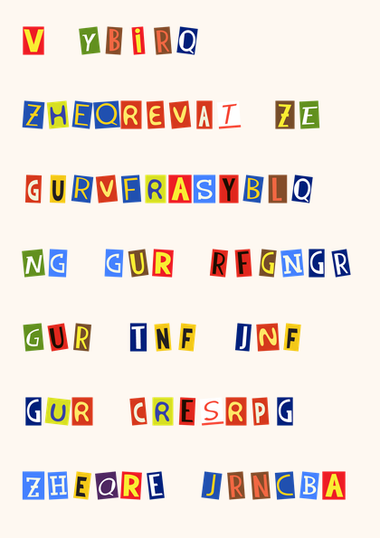
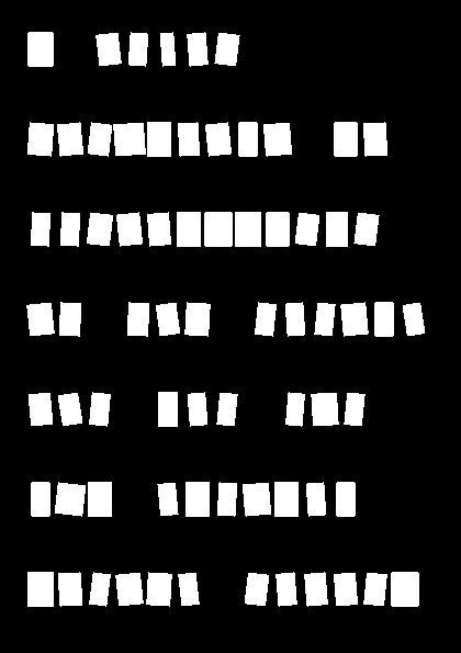
A mask is a binary image that shows where in the color image our "objects" of interest are. For this task, what we are worried about is the location of each letter. In order to measure how well our image segmentation methods perform, we can compare our segmented image to the mask to see how well we segmented each "object"
Task 00: Load Data
Task 00: Description (0 pts.)
Load image data using opencv
For this task, we need to load in the images and corresponding image masks
[Note]: We can use the imread function from the cv2 library to read our images in. We should end up with the actual images shape being (595, 420, 3) and the mask shape being (595, 420).
Images are read in as an array with the format (H, W, C) with the final item being our colors (R, G, B). Since our masks are binary (black and white) we don't need that extra color channel as we can just store 0s or 1s for each of those.
Task 00: Code (0 pts.)
import os
import cv2

import warnings
warnings.filterwarnings("ignore", category=RuntimeWarning)  # all RuntimeWarnings

import numpy as np
import matplotlib.pyplot as plt

# Set random seed for NumPy’s random number generator
#     Conceptually: makes random operations (e.g., random initialization in KMeans, shuffling data, or selecting random samples) produce the same results every time the code is run
#     aka your code becomes reporducable
np.random.seed(42)

# If running on colab and you don't already have the necessary HW data, reclone it
REPO_URL = "https://github.com/nd-cse-30124-fa25/cse-30124-homeworks.git"
REPO_NAME = "cse-30124-homeworks"
HW_FOLDER = "homework03"

try:
    import google.colab

    # Clone repo if not already present
    if not os.path.exists(REPO_NAME):
        !git clone {REPO_URL}

    # cd into the homework folder
    %cd {REPO_NAME}/{HW_FOLDER}

    !git clone https://github.com/rapidsai/rapidsai-csp-utils.git
    !python rapidsai-csp-utils/colab/pip-install.py

except ImportError:
    print('Assignment does not appear to be running on colab, not cloning data repo nor installing CUML')
    print('\t[WARNING]: This means that your SVM will run very, very slowly')
    print('\t[WARNING]: It took me about 25 minutes to run it on my mac mini')
    print('\t[WARNING]: You could install CuML manually')

# Load letters (modify these according to your actual data paths if needed)
image_paths = [f'pages/note_page_{i}.png' for i in range(1, 5)]
mask_paths = [f'pages/mask_page_{i}.png' for i in range(1, 5)]

images = [cv2.cvtColor(cv2.imread(image_path), cv2.COLOR_BGR2RGB) for image_path in image_paths]
masks = [cv2.imread(mask_path, cv2.IMREAD_GRAYSCALE) for mask_path in mask_paths]

print('Image Dimensions:', images[0].shape)
print('Mask Dimensions:', masks[0].shape)
Story Progression
You remember there were a couple of clustering methods in class, but you also remember that typically k-means clustering was the one used as a sort of litmus test, so you figure that may as well be the place to start. Due to the images being so large, if you tried to run agglomerative hierarchical clustering on them you'd crash your kernel 100% of the time (I did this last year).
Task 01: PCA Implementation (3 pts.)
Task 01: Description (0 pts.)
PCA from scratch
[NOTE:] To all three of you that are starting this over fall break, you don't need to actually write this PCA code in order to test everything else. All of the results given below with EV/explained variance set to 0.99/1.0 are essentially equivalent to running the method without PCA. You'll have to comment stuff out but you should be able to test your kmeans and svms just fine without it.
The images are quite large: (595, 420, 3). If you considered every pixel in an image to be a data point, each of our 4 pages has: 595 x 420 x 3 = 749700 "samples" in it! If we can get away with not using all of them we probably should. Towards this end, you will need to implement PCA, which will allow you to reduce the dimensionality of the images while hopefully not losing too much fidelity.
Task 01: Code (3 pts.)
class PCA:
    def __init__(self, n_components=1.0):
        """
        Basic PCA class

        Parameters
        ----------
        n_components:
          - float in (0, 1] -> keep the minimum # of components to reach this
                               fraction of explained variance
        """
        self._expl_var = n_components

    def fit(self, X):
        """
        Fits class to input data

        Parameters
        ----------

        X : array-like, shape (n_samples, n_features)
            Data matrix.
        """

        X = np.asarray(X, dtype=float)
        n_samples, _ = X.shape

        # TODO: Center the data

        # TODO: Use Singular Value Decomposition to get the Singular Values and Explained Variance
        # Hint: numpy has a built in function for calculating SVD

        # TODO: Decide how many components to keep based on n_components

        # Retain only the resolved number of components and related statistics
        self.components_ = Vt[:self._n_components]

        return self

    def transform(self, X):
        """
        Projects the input data into the space defined by the principal components

        Parameters
        ----------
        X : array-like, shape (n_samples, n_features)
            Data matrix.

        Returns
        -------
        Z : array-like, shape (n_samples, self._n_components)
            Data matrix.
        """

        # TODO: Transform the dataset into the new space described by the principal components

        return Z

    def fit_transform(self, X):
        return self.fit(X).transform(X)
Task 02: kmeans Implementation (4 pts.)
Task 02: Description (0 pts.)
kmeans from scratch
One of the most basic clustering methods is kmeans clustering, and it's often used as a first-pass/litmus test when clustering is needed. In the code block below, you're will implement the kmeans algorithm!
Remember that there are 5 steps in kmeans clustering:
- Specify the number of clusters (centroids)
- Randomly select k samples from our data to start as the centroids of our k clusters
- Assign all unchosen samples to the closest cluster based on their euclidian distances to each of the centroids
- After assigning all samples, recalculate the centroid of each cluster by taking the average position of each sample in the cluster
- If the new centroids are close to the old ones the solution is stable, and we can stop, otherwise [repeat steps 3 and 4 with the new centroids]
Due to the rather uncertain nature of what "stable" actually means, we're going to add two arguments to our kmeans: max_iters and tol. We will use tol as the threshold distance for centroid movement and if that is never triggered, we will end after max_iters (You shouldn't need to change the defaults I've set for these).
Task 02: Code (4 pts.)
class kmeans():
    def __init__(self, n_clusters, max_iters=300, tol=1e-4, random_state=None):
        """
        Basic k-means clustering class

        Parameters
        ---------
        n_clusters : int
            Number of clusters.
        max_iters : int
            Maximum iterations per run.
        tol : float
            Convergence tolerance on centroid movement (L2 norm).
        random_state : int or None
            Seed for reproducibility.
        """

        self._n_clusters = n_clusters
        self._max_iters = max_iters
        self._tol = tol
        self._random_state = random_state

    def _init_centroids(self, X):
        """
        Randomly initializes centroids

        Parameters
        ----------

        X : array-like, shape (n_samples, n_features)
            Data matrix.

        Returns
        -------
        X[idx].copy : ndarray, shape (n_clusters,)
            Randomly selected centroids
        """

        rng = np.random.default_rng(self._random_state)
        n_samples, _ = X.shape

        # TODO: Randomly select n_clusters centroids

        return X[idx].copy()

    def fit_predict(self, X):
        """
        Basic k-means clustering.

        Parameters
        ----------
        X : array-like, shape (n_samples, n_features)
            Data matrix.

        Returns
        -------
        np.logical_not(labels.astype(bool)) : ndarray, shape (n_samples,)
            Cluster assignment for each sample
        """
        X = np.asarray(X, dtype=float)

        labels = None
        centroids = None

        # TODO: Initialize centroids

        for _ in range(self._max_iters):
            # TODO: Calculate euclidian distances for each point from the centroids
            # TODO: Assign each sample to the closest centroid

            # TODO: For each cluster that has members, calculate the average position of members
            # TODO: For each cluster that doesn't have members, reseed it to the furthest point
            # TODO: Replace the original Centroids with these new average positions

            # TODO: Calculate the centroid movement and compare to tol

            if shift < self._tol:
                break

        # Flip the foreground and background labels to match the sklearn output
        return np.logical_not(labels.astype(bool))
Task 3: Evaluating Unsupervised Segmentation (4 pts.)
Task 03-1: Description (0 pts.)
Intersection over Union
We'll need to evaluate how well our segmentation methods are doing. We can use the intersection over union (IoU) metric to evaluate how well our segmentation methods are doing.
Intersection over Union (IoU) is defined as the intersection of the predicted mask and the ground truth mask divided by the union of the predicted mask and the ground truth mask.
$$IoU = \frac{TP}{TP + FP + FN}$$
Where TP is the number of true positives, FP is the number of false positives, and FN is the number of false negatives.
Really all this boils down to is looking at how close our predicted labels, if we made every background cluster pixel black, and every foreground cluster pixel 1, is to our ground-truth mask.
Task 03-1: Code (1 pt.)
def calculate_segmentation_metrics(pred, truth, visualize=False):
    """
    Calculate Intersection over Union (IoU) to measure segmentation accuracy

    Args:
        pred: Binary prediction mask (595, 420)
        truth: Binary ground truth mask (595, 420)


    Returns:
        iou: Intersection over Union (IoU) metric
    """
    if visualize:
      # Visualize the masks
      plt.figure(figsize=(10, 5))

      plt.subplot(1, 2, 1)
      plt.title('Prediction Mask')
      plt.imshow(pred, cmap='gray')
      plt.axis('off')

      plt.subplot(1, 2, 2)
      plt.title('Ground Truth Mask')
      plt.imshow(truth, cmap='gray')
      plt.axis('off')

      plt.show()

    # TODO: Calculate intersection and union

    # TODO: calculate IoU (Intersection over Union)
    #    hint: this is also known as the Jaccard index

    return iou
Task 03-2: Description (0 pts.)
Evaluation of Unsupervised Methods
Now that we have a way to measure how well our clustering worked, we should probably evaluate all of our different methods and combinations we could use. In order to test your implementations of PCA and kmeans, we're going to compare them against the versions of them in the sklearn library. It would be pretty cool if your code worked just as well as what people use on the job!
In addition to trying the different implementations, we should probably test a couple different levels of explained variance for PCA to see how they stack up. We're going to test: 0.75, 0.9, and 0.99
One would assume that 0.99 will yield the best results, but it will be interesting to see the differences between them!
[NOTE]: Since there are a lot of different combinations, I included some helper print functions to better format the output (at least on my monitor, which is pretty wide)
Task 03-2: Helper Code (0 pts.)
def header_printer(i):
    print(f"Image {i+1}:")
    print('#' * 80)
    print()
    print(' ' * 25 + 'EV: 0.75' + ' ' * 40 + 'EV: 0.9' + ' ' * 40 + 'EV: 0.99')
    headers = ' ' * 14 + "Student kmeans" + ' ' * 5 + "sklearn kmeans"
    print(headers * 3)

def row_formatter(ious):
    return f'{ious[0]:.4f}' + ' ' * 12 + f'{ious[1]:.4f}' + ' ' * 23
Task 03-2: Code (1 pt.)
from sklearn.preprocessing import StandardScaler

from sklearn.decomposition import PCA as sklearn_pca
from sklearn.cluster import KMeans as sklearn_kmeans

print("\nEvaluating Unsupervised Segmentation Methods...")
print('#' * 80)
print()

# Initialize pca methods and kmeans methods
pca_implementations = {'Student PCA': PCA, 'sklearn PCA': sklearn_pca}
kmeans_implementations = {'Student kmeans': kmeans(n_clusters=2, random_state=42), 'sklearn kmeans': sklearn_kmeans(n_clusters=2, init='random', random_state=42)}

for i, image in enumerate(images):
    header_printer(i)

    for pca_creator, pca_method in pca_implementations.items():
        results = ' ' * 8

        for offset, ev in enumerate([0.75, 0.9, .99]):
            ious = []
            for kmeans_creator, kmeans_method in kmeans_implementations.items():
                # Reshape the image into a 2D array of pixels and 3 color values (RGB)
                pixels = image.reshape(-1, 3)          # reshaped into a 2D array where each row represents a pixel and the columns represent the RGB color channels
                                                    # Note: The -1 means "reshape it into as many rows as needed" (i.e., one row per pixel), and 3 is the number of columns corresponding to the RGB channels

                # TODO: Apply PCA to reduce dimensionality

                # TODO: Perform K-Means clustering, fit Kmeans to data to get cluster labels for each pixel

                # Reshape the labels back to the image shape
                segmented_image = labels.reshape(image.shape[:2])

                # Calculate IoU to evaluate clustering
                ious.append(calculate_segmentation_metrics(segmented_image.astype(bool), masks[i].astype(bool)))

            results += row_formatter(ious)
        print(f"{pca_creator + results}")
    print()
Task 03-2: Expected Output (1 pts.)
Evaluating Unsupervised Segmentation Methods...
################################################################################

Image 1:
################################################################################

                         EV: 0.75                                        EV: 0.9                                        EV: 0.99
              Student kmeans     sklearn kmeans              Student kmeans     sklearn kmeans              Student kmeans     sklearn kmeans
Student PCA        0.8446            0.8446                       0.8464            0.8464                       0.8468            0.8468
sklearn PCA        0.8446            0.8446                       0.8464            0.8464                       0.8468            0.8468

Image 2:
################################################################################

                         EV: 0.75                                        EV: 0.9                                        EV: 0.99
              Student kmeans     sklearn kmeans              Student kmeans     sklearn kmeans              Student kmeans     sklearn kmeans
Student PCA        0.8208            0.8208                       0.8159            0.8158                       0.8160            0.8159
sklearn PCA        0.8208            0.8208                       0.8159            0.8158                       0.8160            0.8159

Image 3:
################################################################################

                         EV: 0.75                                        EV: 0.9                                        EV: 0.99
              Student kmeans     sklearn kmeans              Student kmeans     sklearn kmeans              Student kmeans     sklearn kmeans
Student PCA        0.8012            0.0281                       0.8032            0.0278                       0.8036            0.0278
sklearn PCA        0.8012            0.0281                       0.8032            0.0278                       0.8036            0.0278

Image 4:
################################################################################

                         EV: 0.75                                        EV: 0.9                                        EV: 0.99
              Student kmeans     sklearn kmeans              Student kmeans     sklearn kmeans              Student kmeans     sklearn kmeans
Student PCA        0.8489            0.8489                       0.8509            0.8507                       0.8512            0.8510
sklearn PCA        0.8489            0.8489                       0.8509            0.8507                       0.8512            0.8510
Task 03-3: Short Answer Questions (2 pts.)
Task 03-3-1: Why do you think, for Image 3, the sklearn IoU was so much smaller than the others?
- [ANSWER]
Task 03-3-2: How many features did our feature vectors actually have? What were they?
- [ANSWER]
Story Progression
The unsupervised segmentation seems to work pretty well, but you wonder if a supervised method might work even better. We could probably set this up in a similar way to the clustering task, but instead of using two clusters (foreground and background), we can have two classes (foreground and background).
Luckily the police have manually created a binary mask for us that we can use as labelled data to train our supervised model.
Unluckily, we need to somehow let each pixel know about the surrounding pixels. So we'll need to somehow create a feature vector for each pixel that contains information about the pixel and the surrounding pixels.
Maybe we can take a patch around each pixel and use the RGB values of the pixels in the patch as features?
Task 04: Supervised Image Segmentation
Task 04-1: Description (0 pts.)
Feature Vector Extraction
To train our SVM, we need to create some features. In Homework02 you had to create some features that could describe the evening that a person had, and you used things like time spent in each room and how their activities related to weapons. In this homework, you need to design a feature to describe a pixel. Usually when doing Computer Vision (CV) it's useful for a feature vector for a specific pixel to also include some information about what the surrounding pixels look like.
In the block below, you'll write a function to extract feature vectors for each pixel, taking into account a "patch" of surrounding pixels.
Task 04-1: Code (2 pts.)
def extract_features(image, patch_size=5):
    """
    Extract features for each pixel using RGB values and local neighborhood.

    Args:
        image: RGB image (595, 420, 3)
        patch_size: Size of the local neighborhood patch (must be odd)

    Returns:
        features: Array of shape (n_pixels, n_features) (249900, 78) (595 x 420, 5 x 5 x 3 + 1 x 3)
    """
    height, width, channels = image.shape

    # Add padding to image
    padding = patch_size // 2

    padded = cv2.copyMakeBorder(
        image,
        padding, padding, padding, padding,
        cv2.BORDER_REFLECT
    )

    # TODO: Calculate total number of pixels

    # TODO: Calculate total number of features per pixel

    # TODO: Initialize data structue to store features for all pixels

    # TODO: Loop through pixels and extracts features for each pixel
    #     hint: the feature vector will be all RGB values for every surrounding pixel concatenated with the pixel itself
    #     hint: this results in a 78 dimensional feature vector, for each pixel!
    #     hint: 5 x 5 patch = 25, 3 colors per pixel gives 3 x 25 = 75 + 3 for the pixel itself again gives 78
    #     hint: use current pixel RGB values and the surrounding local patch
    pixel_idx = 0

    # Return feature matrix
    return features
try:
    import cudf
    from cuml.svm import SVC, LinearSVC
except:
    from sklearn.svm import SVC, LinearSVC

# -------------------------------------
# Task 5: SVM Segmentation
# -------------------------------------
def svm_segmentation(model, pca, test_image):
    # TODO: Extract features of testing image

    # TODO: Apply transformations to testing image if PCA != None
    #     hint: transformations means scaling and dimensionality reduction

    # Attempt to move test features to GPU
    try:
        X_test = cudf.DataFrame.from_records(X_test)
    except:
        pass

    # TODO: Predict on test image

    # Attempt to retrieve results from GPU
    try:
        predictions = predictions.to_cupy().get()  # get() brings it to CPU as np.ndarray
    except:
        pass

    # Reshape predictions to match image matrix shape
    segmented_image = predictions.reshape(test_image.shape[:2])

    return segmented_image
Task 04-3: Description (0 pts.)
Properly set colab env
[WARNING]: Colab only gives limited GPU runtime to users, and it takes quite some time to refresh. I would recommend you first test and debug your code with the linear kernel on the CPU environment to first make sure you can actually produce results, and only switch to the GPU environment when you're planning on doing your final run-through.
SVMs are very very slow for large datasets (which these images count as). In order to make your evaluations run faster, we will use an implementation of the SVM that can run on the GPU, making it much more efficient. Colab gives free (limited) access to GPUs. You can follow the steps below to change your environment to be one with a GPU.
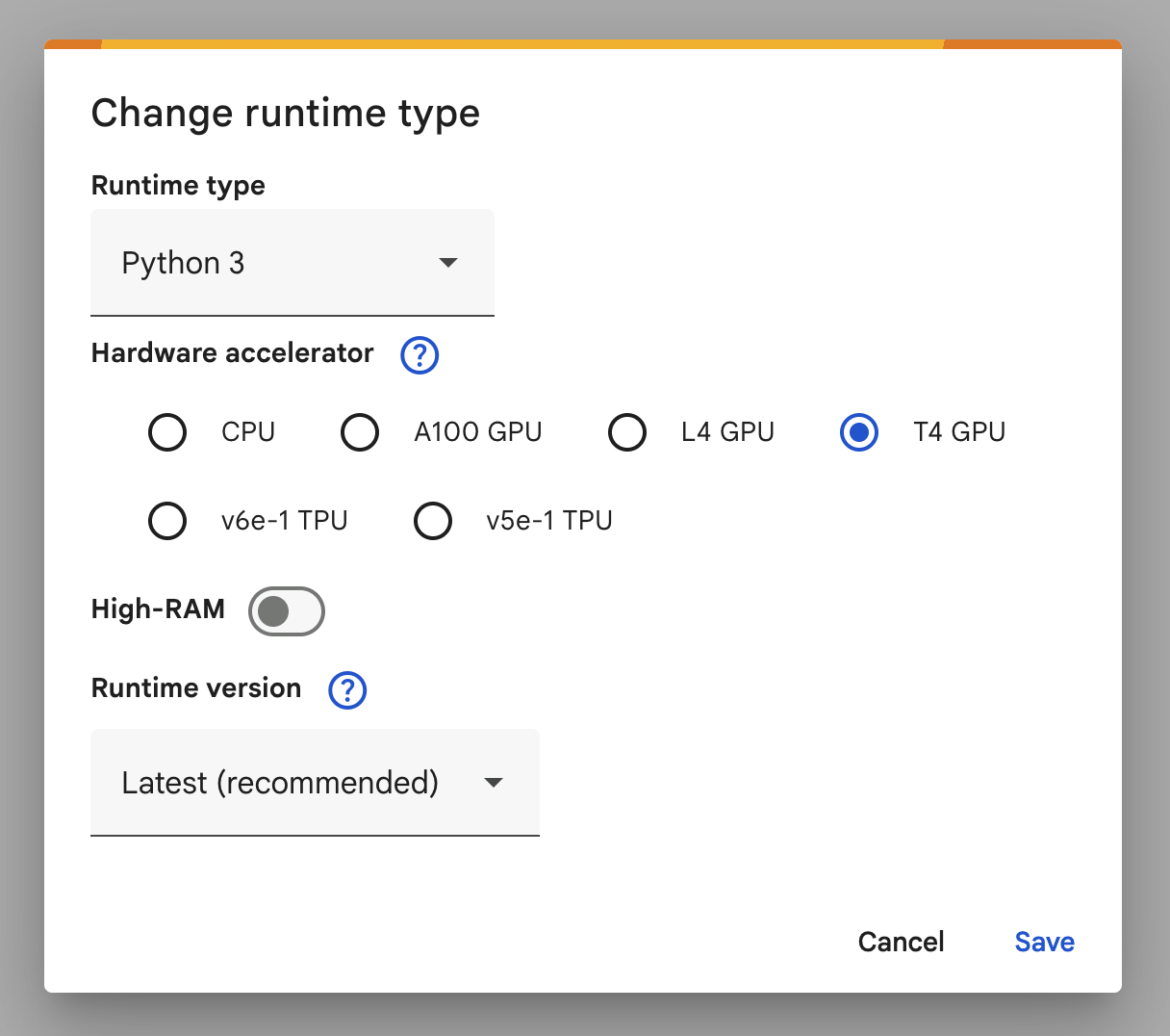
- Select the
Change runtime typefrom the environment dropdown in the upper right
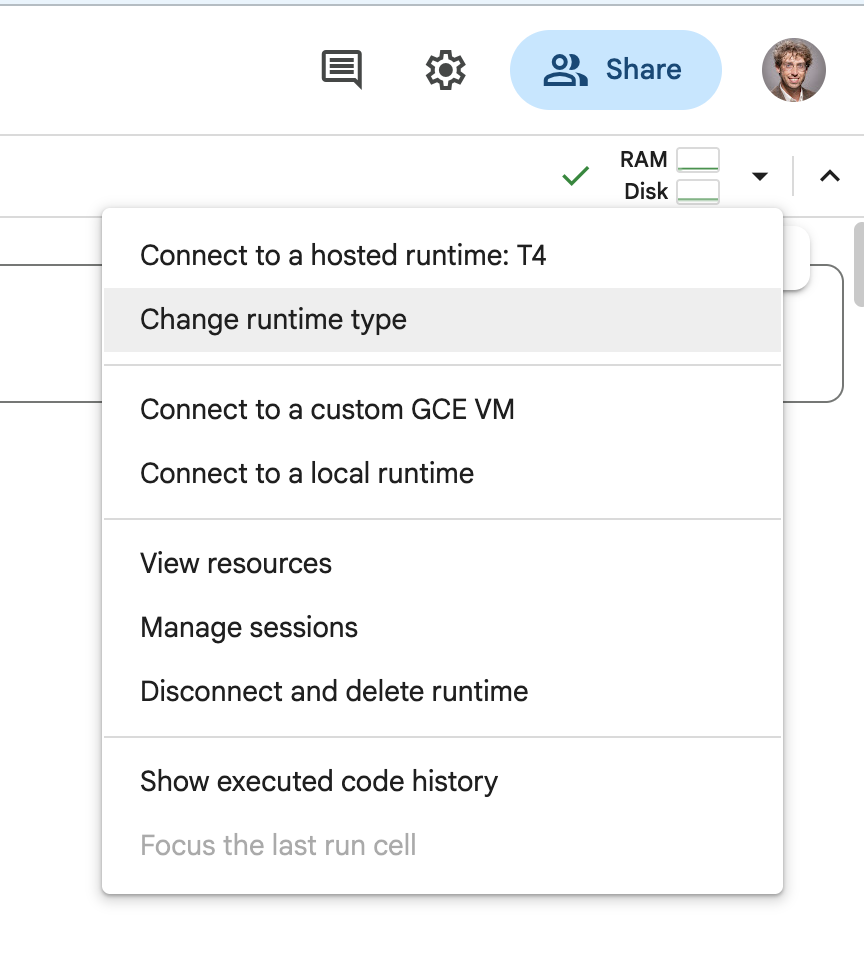
- Select t4 GPU as your environment
[WARNING]: If you're not running this on colab it will likely be very slow. My code took 24m 33.9s to complete on my mac mini in my office and if you're on your laptop it will likely be even slower. You could theoretically install CuML yourself (but it's not compatible with macos for some ungodly reason) if you wanted to work locally by running:
pip install cudf
pip install cuml
Task 04-4: Description (0 pts.)
Supervised Segmentation Evaluation
Much like with the unsupervised segmentation, we have a couple different options that we can tweak for our supervised model. We can try different combinations of kernels and components. You should test [0.75, 0.9, 1.0] for PCA (we will use only your implementation of it) and for the kernels you should test ['linear', 'poly', 'rbf']. Usually rbf is the best one but it's important to actually test it!
Task 04-4: Code (2 pts.)
print("Evaluating Supervised Segmentation Methods...")
print('#' * 80)
print()

# We only use the first 1000 pixels from the training image and mask, otherwise it takes too long to train
# We'll train on only the first 1000 pixels from the first image, and test only on the second (again for sake of runtimes)
# Really we should be doing some 4 fold cross validation with full images here but I don't want to wait 9 hours for it to run
train_image = images[0][:1000]
train_mask = masks[0][:1000]

test_image = images[1]
test_mask = masks[1]

# TODO: Extract features of training image

y_train = (train_mask > 0).reshape(-1)

# TODO: Declare the kernels we want to test
for kernel in []:
    print(f"Testing an SVM with a {kernel} kernel:")

    # TODO: Declare the explained variances we want to test
    for ev in []:
        # TODO: Apply PCA

        # Attempt to move to GPU (as cuDF)
        try:
            X_train_pca = cudf.DataFrame.from_records(X_train_pca)
            y_train = cudf.Series(y_train)
        except:
            pass

        # TODO: Initialize the SVM using LinearSVC for the linear kernel and SVC for everything else

        # TODO: Fit the SVM to the training data

        # TODO: segment the test image and calculate the IoU for it compared to the test mask

        print(f"\tAn explained variance of {ev} results in an IoU of {iou:.2f}")

    print()
    print('#' * 80)
    print()
Task 04-3: Expected Output (1 pt.)
Evaluating Supervised Segmentation Methods...
################################################################################

Testing an SVM with a linear kernel:
	An explained variance of 0.75 results in an IoU of 0.82
	An explained variance of 0.9 results in an IoU of 0.83
	An explained variance of 1.0 results in an IoU of 0.86

################################################################################

Testing an SVM with a poly kernel:
	An explained variance of 0.75 results in an IoU of 0.84
	An explained variance of 0.9 results in an IoU of 0.89
	An explained variance of 1.0 results in an IoU of 0.93

################################################################################

Testing an SVM with a rbf kernel:
	An explained variance of 0.75 results in an IoU of 0.90
	An explained variance of 0.9 results in an IoU of 0.95
	An explained variance of 1.0 results in an IoU of 0.98

################################################################################
Task 04-4: Short Answer Questions (2 pts.)
Task 04-4-1: What is it about SVMs that make them very slow (Hint: It has to do with the dual-form equation)?
- [ANSWER]
Task 04-4-2: Do you think increasing the patch size of our features would make our results better?
- [ANSWER]
Task 05: Region Extraction
Task 05-1: Description (0 pts.)
Region localization from SVM image segmentation
Now that we have a best model, we can actually segment our pages and extract each letter! This computer vision stuff is outside the scope of this course, so the code is just provided for you. But this is how we can extract the region of each letter using our segmentation!
Task 05-1: Code (0 pts.)
from skimage.measure import label, regionprops
import os

def extract_and_save_letters(segmented_image, original_image, page, output_dir='letters'):
    """
    Extract each segmented letter and save as a separate PNG file.

    Args:
        segmented_image: Segmented image with unique labels for each letter
        original_image: Original RGB image
        output_dir: Directory to save the extracted letter images
    """
    # Ensure the output directory exists
    os.makedirs(output_dir, exist_ok=True)

    # Label connected components
    labeled_image = label(segmented_image)

    # Iterate over each labeled region
    for region in regionprops(labeled_image):
        # Extract the bounding box of the region
        min_row, min_col, max_row, max_col = region.bbox

        # Extract the region from the original image
        letter_image = original_image[min_row:max_row, min_col:max_col]

        # Save the extracted letter as a PNG file
        letter_filename = os.path.join(output_dir, f'note_{page}_letter_{region.label}.png')
        cv2.imwrite(letter_filename, cv2.cvtColor(letter_image, cv2.COLOR_RGB2BGR))
# Attempt to move to GPU (as cuDF)
try:
    X_train = cudf.DataFrame.from_records(X_train)
    y_train = cudf.Series(y_train)
except:
    pass

svm = SVC(kernel='rbf')
svm.fit(X_train, y_train)

for page, image in enumerate(images):
    segmented_image = svm_segmentation(svm, None, image)
    extract_and_save_letters(segmented_image, image, page)
Task 05-2: Example Output (0 pts.)
Since there are 262 characters across all 4 pages of the note, I won't show all of the output, but here are the letters my code extracted from the first line of the first page:


Story Progression
WOW! We did it, we used AI to take in an image of a ransom note, figure out where each individual letter was, and created a cropped image of each one!
Now that we have all of the letters extracted, we can perform Optical Character Recognition (OCR) on each letter. OCR is the process of taking in a picture of a character and returning the actual ascii character it represents (think MNIST).
While the police want the data ASAP, you know you need a break for a lil drinky-poo. The police will have to wait, but in the next homework you'll explore how to do OCR on your extracted letters with a basic Feed-Forward Neural Network (which you'll be writing from scratch) and a Convolutional Neural Network (which you'll be using from PyTorch).